Simulation flow

In every molecular simulation, the main steps are roughly the same. We start by setting the simulated system: positions of the particles, maybe velocities, atomic types, potential to use between the atoms, etc. Secondly, we have to choose the simulation type and setup the propagator and the analysis algorithms.

Then we can run the simulation for a given number of steps nsteps. During the run, the propagator can be a Newton integrator for Molecular Dynamics, a MonteCarlo propagator for MonteCarlo simulation, a Gradient descent for energy minimization, etc. Other algorithms can be added to the simulation, in order to perform live analysis of the simulation or to output data.

All this is summarised in the figure Simulation flow in Jumos.

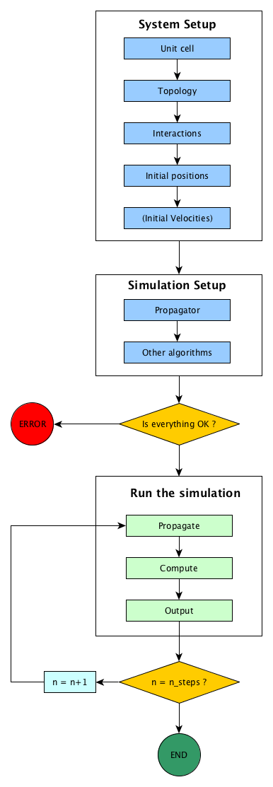
Simulation flow in Jumos

All the steps in the process of running a simulation are described below.

System setup

The system will contain all the physical informations about what we are simulating. In Jumos, a system is represented by the Universe type. It should at least contain data about the simulation cell, the system topology, the initial particles coordinates and the interactions between the particles.

Simulation setup

During the simulation, the system will be propagated by a propagator: MolecularDynamics, MonteCarlo, Minimization are examples of propagators. Other algorithms can take place here, either algorithms to compute thermodynamic properties or algorithms to modify the behaviour of the simulation.

Running the simulation

The simulation run is the main part of the simulation, and consist in three main steps:

• Use the propagator to genrerate an update in the particles positions;
• Compute thermodynamical properties of the system;
• Output data to file for later analysis.