Usual simulation steps
Note
All the capacities presented here may not be implemented (at least not yet) in Jumos. However, this page describes the exact steps involved in preparing and running a simulation with Jumos.
In every molecular dynamics simulation, the main steps are roughly the same. One shall start by setting the simulation : positions of the particles, velocities (either from a file or from a random gaussian distribution), timestep, atomic types, potential to use between the atoms, and so on.
Then we can run the simulation for a given number of steps n_steps. During the
run, the three main steps are: computing the forces from the potentials;
integrating the movement and outputing the quantities of interest : trajectories,
energy, temperature, pressure, etc.
This is summarised in the figure Usual steps in a molecular dynamic simulation.
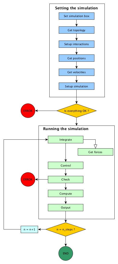
Usual steps in a molecular dynamic simulation
Setting the simulation
Here, one is building his simulation. The order of the steps doesn’t matter: we should start by defining the simulation cell, and we have to define a topology before setting the initial positions, but we may setup the interactions at any time.
Get topology
The topology of a simulation is a representation of the atoms, molecules, groups
of molecules found in this simulation. It can be read from a file
(.pdb files ,:file:.lmp LAMMPS topology, …) ; guessed from the initial
configuration (two atoms are linked if they are closer than the sum of there Van
der Waals radii) ; or built by hand.
Setup interaction
The interactions describe how atoms should behave: they can be pair potentials, many-body potentials, bond potentials, torsion potentials, dihedral potentials or any other kinds of interactions.
Each of these potentials is associated with a force. This force is used in molecular dynamics to integrate Newton’s equations of motions.
Initial positions
The initial positions of all the atoms in the system can be read from a file, or defined by hand.
Initial velocities
We will also need the initial velocities to start the time integration in molecular dynamics. They can be defined either in a file (to restart previous dynamic), or randomly assigned. In the later case, it is better to use a Maxwell-Boltzmann distribution at the temperature \(T\) of the simulation.
Setup simulation
We will have to set other values in order to run a simulation, depending on the kind of simulation: the timestep of integration \(dt\), the type of thermostat or barostat to use.
Running the simulation
The order of the steps in a simulation run is fixed, and can not be changed.
Integrate
Using the forces, one can now integrate Newton’s equations of motions. Numerous algorithms exist, such as velocity-Verlet, Beeman algorithm, multi-timestep RESPA algorithm. At the end, postions and velocities are updated to the new step.
Get forces
During the integration steps, we will need forces acting on the atoms. This forces computing step is the most time consuming aspect of the calculation. Various ways to do this computation exists, depending on the type of potentials (short range or long range, bonding or not bonding), and some tricks can speed up this computation (pairs list, short range potential truncation).
The algorithm used for integration have to call this step when and as many times as needed.
Control
If the time integration does not force the value of external parameters, like temperature or pressure or volume, this step can enforce them. Controls examples are the Berendsen thermostat, velocity rescaling, particle wrapping to the cell.
Check
During the run, one can check for simulation consistency. For example, the number of particles in the cell may have be constant, the global momentum should be null, and so on.
Compute
This step allows for computing and averaging physical quantities, such as total energy, kinetic energy, temperature, pressure, magnetic moment, and any other physical quantities.
Output
In order to exploit the computation results, we have to do save them to a file. during this step, we can output computed values and the trajectory.